A Wald/Score chi-square test can be used for continuous and categorical variables. Whereas, Pearson chi-square is used for categorical variables. The p-value indicates whether a coefficient is significantly different from zero. In logistic regression, we can select top variables based on their high wald chi-square value.
Gain :Gain at a given decile level is the ratio of cumulative number of targets (events) up to that decile to the total number of targets (events) in the entire data set. This is also called CAP (Cumulative Accuracy Profile) in Finance, Credit Risk Scoring Technique
Interpretation: % of targets (events) covered at a given decile level. For example, 80% of targets covered in top 20% of data based on model. In the case of propensity to buy model, we can say we can identify and target 80% of customers who are likely to buy the product by just sending email to 20% of total customers.
Interpretation: The Cum Lift of 4.03 for top two deciles, means that when selecting 20% of the records based on the model, one can expect 4.03 times the total number of targets (events) found by randomly selecting 20%-of-file without a model.
- Randomly split data into two samples: 70% = training sample, 30% = validation sample.
- Score (predicted probability) the validation sample using the response model under consideration.
- Rank the scored file, in descending order by estimated probability
- Split the ranked file into 10 sections (deciles)
- Number of observations in each decile
- Number of actual events in each decile
- Number of cumulative actual events in each decile
- Percentage of cumulative actual events in each decile. It is called Gain Score.
- Divide the gain score by % of data used in each portion of 10 bins. For example, in second decile, divide gain score by 20.
| Decile Rank | Number of cases | Number of Responses | Cumulative Responses | % of Events | Gain | Cumulative Lift | Number of Decile Score to divide Gain |
| 1 | 2500 | 2179 | 2179 | 44.71% | 44.71% | 4.47% | 10 |
| 2 | 2500 | 1753 | 3932 | 35.97% | 80.67% | 4.03% | 20 |
| 3 | 2500 | 396 | 4328 | 8.12% | 88.80% | 2.96% | 30 |
| 4 | 2500 | 111 | 4439 | 2.28% | 91.08% | 2.28% | 40 |
| 5 | 2500 | 110 | 4549 | 2.26% | 93.33% | 1.87% | 50 |
| 6 | 2500 | 85 | 4634 | 1.74% | 95.08% | 1.58% | 60 |
| 7 | 2500 | 67 | 4701 | 1.37% | 96.45% | 1.38% | 70 |
| 8 | 2500 | 69 | 4770 | 1.42% | 97.87% | 1.22% | 80 |
| 9 | 2500 | 49 | 4819 | 1.01% | 98.87% | 1.10% | 90 |
| 10 | 2500 | 55 | 4874 | 1.13% | 100.00% | 1.00% | 100 |
| 25000 | 4874 |

Detecting Outliers
1. Box Plot Method : If a value is higher than the 1.5*IQR above the upper quartile (Q3), the value will be considered as outlier. Similarly, if a value is lower than the 1.5*IQR below the lower quartile (Q1), the value will be considered as outlier.
QR is interquartile range. It measures dispersion or variation. IQR = Q3 -Q1.Some researchers use 3 times of interquartile range instead of 1.5 as cutoff. If a high percentage of values are appearing as outliers when you use 1.5*IQR as cutoff, then you can use the following rule
Lower limit of acceptable range = Q1 - 1.5* (Q3-Q1)
Upper limit of acceptable range = Q3 + 1.5* (Q3-Q1)
Lower limit of acceptable range = Q1 - 3* (Q3-Q1)
Upper limit of acceptable range = Q3 + 3* (Q3-Q1)
Acceptable Range : The mean plus or minus three Standard Deviation
- The mean and standard deviation are strongly affected by outliers.
- It assumes that the distribution is normal (outliers included)
- It does not detect outliers in small samples
4. Weight of Evidence: Logistic regression model is one of the most commonly used statistical technique for solving binary classification problem. It is an acceptable technique in almost all the domains. These two concepts - weight of evidence (WOE) and information value (IV) evolved from the same logistic regression technique. These two terms have been in existence in credit scoring world for more than 4-5 decades. They have been used as a benchmark to screen variables in the credit risk modeling projects such as probability of default. They help to explore data and screen variables. It is also used in marketing analytics project such as customer attrition model, campaign response model etc.
What is Weight of Evidence (WOE)?
The weight of evidence tells the predictive power of an independent variable in relation to the dependent variable. Since it evolved from credit scoring world, it is generally described as a measure of the separation of good and bad customers. "Bad Customers" refers to the customers who defaulted on a loan. and "Good Customers" refers to the customers who paid back loan.
Distribution of Goods - % of Good Customers in a particular group
Distribution of Bads - % of Bad Customers in a particular groupln - Natural LogPositive WOE means Distribution of Goods > Distribution of Bads
Negative WOE means Distribution of Goods < Distribution of BadsHint : Log of a number > 1 means positive value. If less than 1, it means negative value.
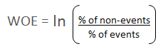
Weight of Evidence was originated from logistic regression technique. It tells the predictive power of an independent variable in relation to the dependent variable. It is calculated by taking the natural logarithm (log to base e) of division of % of non-events and % of events.
Outlier Treatment with Weight Of Evidence : Outlier classes are grouped with other categories based on Weight of Evidence (WOE).
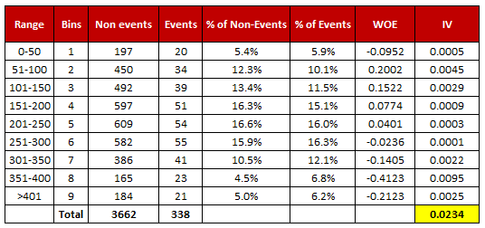
- For a continuous variable, split data into 10 parts (or lesser depending on the distribution).
- Calculate the number of events and non-events in each group (bin)
- Calculate the % of events and % of non-events in each group.
- Calculate WOE by taking natural log of division of % of non-events and % of events

WEIGHT OF EVIDENCE (WOE) AND INFORMATION VALUE (IV) EXPLAINED
Logistic regression model is one of the most commonly used statistical technique for solving binary classification problem. It is an acceptable technique in almost all the domains. These two concepts - weight of evidence (WOE) and information value (IV) evolved from the same logistic regression technique. These two terms have been in existence in credit scoring world for more than 4-5 decades. They have been used as a benchmark to screen variables in the credit risk modeling projects such as probability of default. They help to explore data and screen variables. It is also used in marketing analytics project such as customer attrition model, campaign response model etc.
What is Weight of Evidence (WOE)?
The weight of evidence tells the predictive power of an independent variable in relation to the dependent variable. Since it evolved from credit scoring world, it is generally described as a measure of the separation of good and bad customers. "Bad Customers" refers to the customers who defaulted on a loan. and "Good Customers" refers to the customers who paid back loan. |
| WOE Calculation |
Distribution of Goods - % of Good Customers in a particular group
Distribution of Bads - % of Bad Customers in a particular group
ln - Natural Log
Negative WOE means Distribution of Goods < Distribution of Bads
Hint : Log of a number > 1 means positive value. If less than 1, it means negative value.
WOE = In(% of non-events ➗ % of events)
 |
| Weight of Evidence Formula |
Steps of Calculating WOE
- For a continuous variable, split data into 10 parts (or lesser depending on the distribution).
- Calculate the number of events and non-events in each group (bin)
- Calculate the % of events and % of non-events in each group.
- Calculate WOE by taking natural log of division of % of non-events and % of events
 |
| Weight of Evidence and Information Value Calculation |
Terminologies related to WOE
1. Fine Classing : Create 10/20 bins/groups for a continuous independent variable and then calculates WOE and IV of the variableFor continuous independent variables : First, create bins (categories / groups) for a continuous independent variable and then combine categories with similar WOE values and replace categories with WOE values. Use WOE values rather than input values in your model.
WEIGHT OF EVIDENCE (WOE) AND INFORMATION VALUE (IV) EXPLAINED
Logistic regression model is one of the most commonly used statistical technique for solving binary classification problem. It is an acceptable technique in almost all the domains. These two concepts - weight of evidence (WOE) and information value (IV) evolved from the same logistic regression technique. These two terms have been in existence in credit scoring world for more than 4-5 decades. They have been used as a benchmark to screen variables in the credit risk modeling projects such as probability of default. They help to explore data and screen variables. It is also used in marketing analytics project such as customer attrition model, campaign response model etc.
What is Weight of Evidence (WOE)?
The weight of evidence tells the predictive power of an independent variable in relation to the dependent variable. Since it evolved from credit scoring world, it is generally described as a measure of the separation of good and bad customers. "Bad Customers" refers to the customers who defaulted on a loan. and "Good Customers" refers to the customers who paid back loan. |
| WOE Calculation |
Distribution of Goods - % of Good Customers in a particular group
Distribution of Bads - % of Bad Customers in a particular group
ln - Natural Log
Negative WOE means Distribution of Goods < Distribution of Bads
Hint : Log of a number > 1 means positive value. If less than 1, it means negative value.
WOE = In(% of non-events ➗ % of events)
|
| Weight of Evidence Formula |
Steps of Calculating WOE
- For a continuous variable, split data into 10 parts (or lesser depending on the distribution).
- Calculate the number of events and non-events in each group (bin)
- Calculate the % of events and % of non-events in each group.
- Calculate WOE by taking natural log of division of % of non-events and % of events
|
| Weight of Evidence and Information Value Calculation |
Download : Excel Template for WOE and IV
Terminologies related to WOE
1. Fine ClassingCreate 10/20 bins/groups for a continuous independent variable and then calculates WOE and IV of the variable2. Coarse Classing
Combine adjacent categories with similar WOE scores
Usage of WOE
Weight of Evidence (WOE) helps to transform a continuous independent variable into a set of groups or bins based on similarity of dependent variable distribution i.e. number of events and non-events.For continuous independent variables : First, create bins (categories / groups) for a continuous independent variable and then combine categories with similar WOE values and replace categories with WOE values. Use WOE values rather than input values in your model.
Categorical independent variables: Combine categories with similar WOE and then create new categories of an independent variable with continuous WOE values. In other words, use WOE values rather than raw categories in your model. The transformed variable will be a continuous variable with WOE values. It is same as any continuous variable.
It is because the categories with similar WOE have almost same proportion of events and non-events. In other words, the behavior of both the categories is same.Why combine categories with similar WOE?
- Each category (bin) should have at least 5% of the observations.
- Each category (bin) should be non-zero for both non-events and events.
- The WOE should be distinct for each category. Similar groups should be aggregated.
- The WOE should be monotonic, i.e. either growing or decreasing with the groupings.
- Missing values are binned separately.
FEATURE SELECTION : SELECT IMPORTANT VARIABLES WITH BORUTA PACKAGE
Why Variable Selection is important?
- Removing a redundant variable helps to improve accuracy. Similarly, inclusion of a relevant variable has a positive effect on model accuracy.
- Too many variables might result to overfitting which means model is not able to generalize pattern
- Too many variables leads to slow computation which in turns requires more memory and hardware.
Why Boruta Package?
There are a lot of packages for feature selection in R. The question arises " What makes boruta package so special". See the following reasons to use boruta package for feature selection.
- It works well for both classification and regression problem.
- It takes into account multi-variable relationships.
- It is an improvement on random forest variable importance measure which is a very popular method for variable selection.
- It follows an all-relevant variable selection method in which it considers all features which are relevant to the outcome variable. Whereas, most of the other variable selection algorithms follow a minimal optimal method where they rely on a small subset of features which yields a minimal error on a chosen classifier.
- It can handle interactions between variables
- It can deal with fluctuating nature of random a random forest importance measure
Perform shuffling of predictors' values and join them with the original predictors and then build random forest on the merged dataset. Then make comparison of original variables with the randomised variables to measure variable importance. Only variables having higher importance than that of the randomised variables are considered important.
Follow the steps below to understand the algorithm -
- Create duplicate copies of all independent variables. When the number of independent variables in the original data is less than 5, create at least 5 copies using existing variables.
- Shuffle the values of added duplicate copies to remove their correlations with the target variable. It is called shadow features or permuted copies.
- Combine the original ones with shuffled copies
- Run a random forest classifier on the combined dataset and performs a variable importance measure (the default is Mean Decrease Accuracy) to evaluate the importance of each variable where higher means more important.
- Then Z score is computed. It means mean of accuracy loss divided by standard deviation of accuracy loss.
- Find the maximum Z score among shadow attributes (MZSA)
- Tag the variables as 'unimportant' when they have importance significantly lower than MZSA. Then we permanently remove them from the process.
- Tag the variables as 'important' when they have importance significantly higher than MZSA.
- Repeat the above steps for predefined number of iterations (random forest runs), or until all attributes are either tagged 'unimportant' or 'important', whichever comes first.
Major Disadvantages: Boruta does not treat collinearity while selecting important variables. It is because of the way algorithm works.
In Linear Regression:
There are two important metrics that helps evaluate the model - Adjusted R-Square and Mallows' Cp Statistics.Adjusted R-Square: It penalizes the model for inclusion of each additional variable. Adjusted R-square would increase only if the variable included in the model is significant. The model with the larger adjusted R-square value is considered to be the better model.
A final model should be selected based on the following two criteria's -
First Step : Models in which number of variables where Cp is less than or equal to p
Important Note :
For parameter estimation, Hocking recommends a model where Cp<=2p – pfull +1, where p is the number of parameters in the model, including the intercept. pfull - total number of parameters (initial variable list) in the model.
- Pearson correlation is a measure of linear relationship. The variables must be measured at interval scales. It is sensitive to outliers. If pearson correlation coefficient of a variable is close to 0, it means there is no linear relationship between variables.
- Spearman's correlation is a measure of monotonic relationship. It can be used for ordinal variables. It is less sensitive to outliers. If spearman correlation coefficient of a variable is close to 0, it means there is no monotonic relationship between variables.
- Hoeffding’s D correlation is a measure of linear, monotonic and non-monotonic relationship. It has values between –0.5 to 1. The signs of Hoeffding coefficient has no interpretation.
If a variable has a very low rank for Spearman (coefficient - close to 0) and a very high rank for Hoeffding indicates a non-monotonic relationship.
If a variable has a very low rank for Pearson (coefficient - close to 0) and a very high rank for Hoeffding indicates a non-linear relationship.